Example: Basic
Test Scenario Definition
This test scenario is designed to evaluate the network’s performance and robustness under high traffic load conditions, specifically focusing on the interaction between high-volume UDP traffic and HTTP traffic. The scenario forms the basics for modeling a realistic network environment where various types of data flows coexist and compete for bandwidth and network resources, which is typical in enterprise networks or service provider environments.
This configuration includes the following traffic types:
UDP Traffic: Simulates heavy background traffic from a NSI to a CPE, intended to create network congestion.
Bidirectional HTTP Traffic: Runs in parallel with the UDP traffic, representing typical web traffic between NSI and CPE (both directions), to assess the network’s ability to handle regular web services amidst congestion.
Note
The traffic endpoint on the CPE side can be either a ByteBlower Port or a ByteBlower Endpoint.
This scenario aims to understand how high-volume background traffic (UDP) impacts the performance and reliability of standard web traffic (HTTP), focusing on metrics like latency, retransmissions, and throughput. The results will offer insights into the network’s capacity and efficiency, guiding optimization for a balanced and resilient network performance.
Tip
The ByteBlower Test Framework makes it easy to run flows in both directions. Just turn on the reverse flow option in the settings of the original flow:
{
    "add_reverse_direction": true
}
Activating such a reverse flow is available for all types of flows.
Run a test
Using the ByteBlower Test Framework, the traffic test scenario can be run via command-line interface. You can use the following steps:
Create a working directory and (preferably) a Python virtual environment within.
Activate the virtual environment and install the ByteBlower Test Framework.
Copy one of these example files into your working directory (based on what you want to test):
Update the example file to your own test setup (ByteBlower server, port/endpoint configuration, etc.)
Run the test from your working directory using the command line interface:
byteblower-test-framework
python -m byteblower_test_framework
More details regarding these steps are given in Installation & Quick start.
Result Highlights
In this section, we explain the structure of the HTML report, and how to interpret the findings.
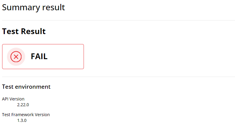
Test status & environment
The first part of the report contains the overall test status, which indicates whether the network performance met or failed the predefined requirements. These requirements typically include maximum tolerated packet loss and latency thresholds, among others. A test is considered as failed if at least one flow status is FAIL (the actual failure cause(s) are indicated in the individual flow results).
The test environment section provides essential details on the API and the ByteBlower Test Framework versions used for the test. In this instance, API version 2.22.0 and ByteBlower Test Framework version 1.3.0 were used.
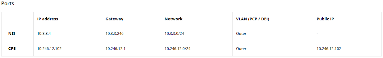
Ports and config
Next, you will find the port configuration table that outlines the setup of the network ports involved in the test, including IP addresses, network masks, gateways, etc.
Correlated test results
The report then presents the correlated test results, which aggregate the throughput and latency CCDF results (when latency analysis is enabled) for UDP flows (we do not support aggregating HTTP flow results yet). When multiple flows are used, this section starts with a summary throughput graph for each port involved in transmission and reception. Then, it presents the aggregated latency CCDF results of all UDP flows. In this case, there is only the aggregated CCDF since only one UDP flow is configured.
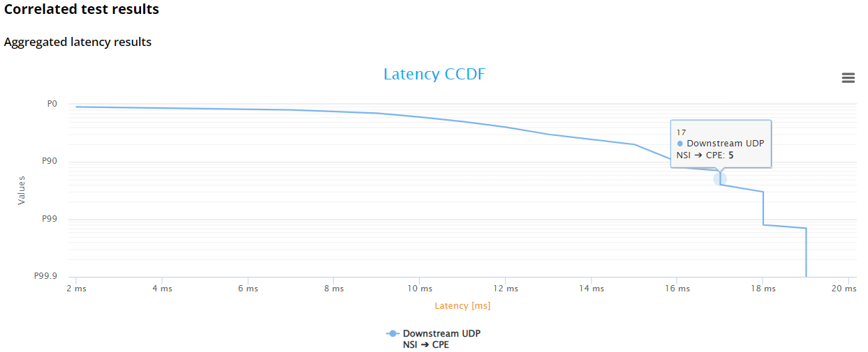
The CCDF graph indicates the percentage of packets with latencies below or above specific latency values. In this scenario, for example, 95% of packets have latencies under 17ms.
Individual test results
The individual test results part contains the following information:
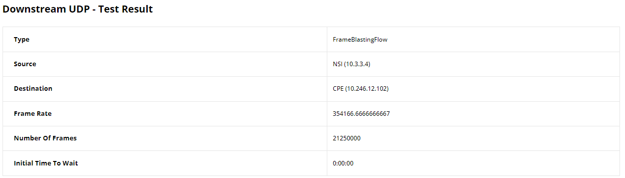
UDP Frame Blasting Test Results
This section provides comprehensive result statistics for the UDP traffic analysis. It starts with a table displaying the configuration of the UDP flow, including source and destination details, frame rate, and the number of frames. This information serves as a reminder of the configuration to better understand the flow’s behavior during the test.
When latency analysis is enabled for this flow, you will find the results of the Frame Latency CDF and Loss Analyser, which details the performance of the UDP traffic. We first have the test status (which is FAIL in this case) in addition to failure cause(s).
Then, it reports critical statistics such as the number of packets transmitted and received, the total bytes, any losses incurred, and latency figures including minimum, maximum, average, average latency jitter (variation in time delay between packets), and the number of packets below/above latency histogram thresholds. These results are pivotal for diagnosing issues related to packet timing and network congestion.
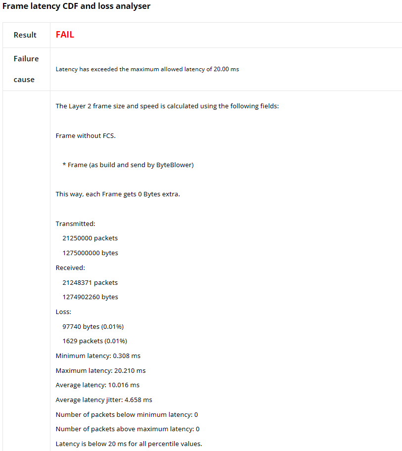
Accompanying the previous data are the Latency CDF/CCDF graphs. The Latency CDF graph plots present the percentage of latency falling below a given threshold, offering a perspective on the overall latency distribution. Meanwhile, the Latency CCDF graph complements this by illustrating the latency distribution, to identify the proportion of packets experiencing latencies that are lower/higher than certain latency values for understanding the quality of service for time-sensitive applications.

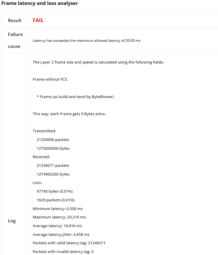
Next, the results from the Frame Latency and Loss Analyser are presented. This section offers a summary of key performance statistics similar to the previous one, with a small difference, it provides the number of packets with (in)valid latency tags instead of the number of packets below/above latency thresholds.
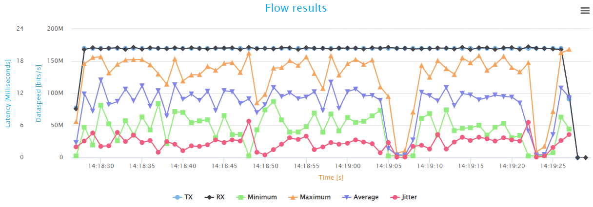
Finally, the report features a graph that illustrates the variation over time of the Tx/Rx throughput, minimum/maximum/average latency, and jitter, providing a visual depiction of the network’s behavior during the test, and an indicator of network stability and performance.
Note
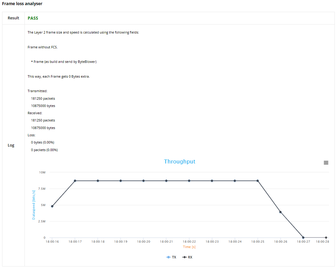
If latency analysis is not enabled, you will find the Frame loss analyser results that highlight transmission/reception and frame loss statistics, in addition to the throughput graph (in transmission and reception).
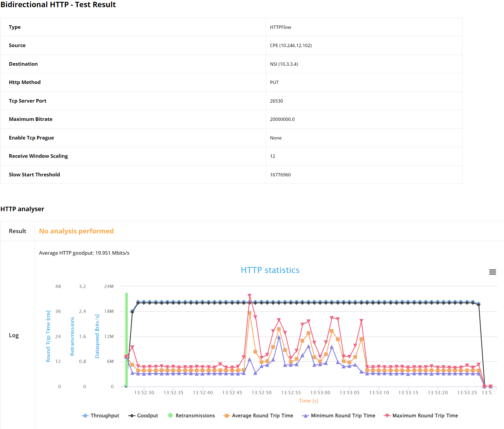
Bidirectional HTTP Test Results
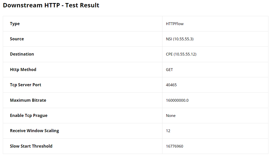
This section presents the results of the HTTP traffic analysis. The information begins with a configuration table of the HTTP flow, detailing the source and destination addresses, the HTTP method used (GET), the TCP server port, and other settings such as the maximum bitrate and TCP window scaling factors. These details provide the context needed to evaluate the HTTP traffic performance within the test.
The results structure of the reverse flow is similar to the original one.
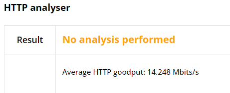
Currently, we do not provide post-processing of HTTP test results. That’s why it is shown No analysis performed in the report (and nor average goodput is calculated).
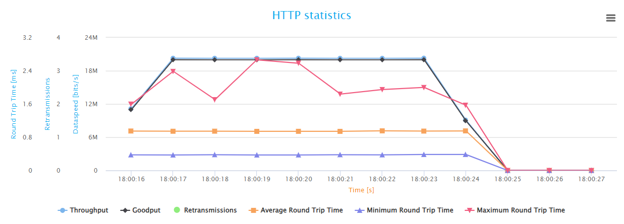
Finally, the HTTP Statistics graph illustrates key performance metrics such as throughput, goodput, retransmissions, and round-trip time, providing insight into the network’s efficiency and stability in handling web traffic. The goodput shows the actual application-level throughput, retransmissions point to loss or errors, while round-trip time indicates the network’s latency.
Note
The same type of results are also included for the HTTP flow in the reverse direction.